How to Use VLOOKUP in Excel? A Step-by-Step Guide with Examples

Microsoft Excel is a deceptively powerful tool for data management. It helps users analyze and interpret data easily. Often not appreciated for the range of tasks it lets the user perform, Microsoft Excel is undoubtedly a powerful and very popular tool used by almost every organization, even today.

Excel provides an extensive range of functions that makes it easier to work with data. VLOOKUP in Excel is one such function. VLOOKUP works as a search function by looking for specific data vertically across a table or spreadsheet.

Let’s go ahead and understand what exactly VLOOKUP in Excel is.

https://youtube.com/watch?v=dn6jnFS3tvg%3Fenablejsapi%3D1%26origin%3Dhttps%253A%252F%252Fwww.simplilearn.com

VLOOKUP Formula

We can use the VLOOKUP function with the help of a simple syntax. The Syntax for VLOOKUP is:

=VLOOKUP(lookup_value, table_array, col_index_number,[range_lookup])

Where, 

• lookup_value: This specifies the value that you want to look up in our data.
• table_array: This is the location where the values are present in excel.
• col_index_number: This specifies the column number from where we need to return the value.
• range_lookup: This has two options; if the value is set to FALSE, that means we are looking for an exact match. If the value is TRUE, then we are looking for an approximate match.

What is VLOOKUP in Excel?

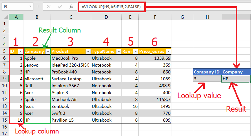
VLOOKUP stands for Vertical Lookup. As the name specifies, VLOOKUP is a built-in Excel function that helps you look for a specified value by searching for it vertically across the sheet. VLOOKUP in Excel may sound complicated, but you will find out that it is a very easy and useful tool once you try it. Look at the example below to understand VLOOKUP.

The VLOOKUP formula below looks for a Company name with Company ID 3.

In the next section, you will understand how to use the VLOOKUP function. 

How To Find an Exact Match Using VLOOKUP?

VLOOKUP makes it effortless to look for an exact match from the table. Let’s take a look at how to do this with the help of an example:

• In the example below, we are using the VLOOKUP function to find the value of the exact match of ID from the given table. So, we set the first parameter as the lookup value, which is the cell H5. 

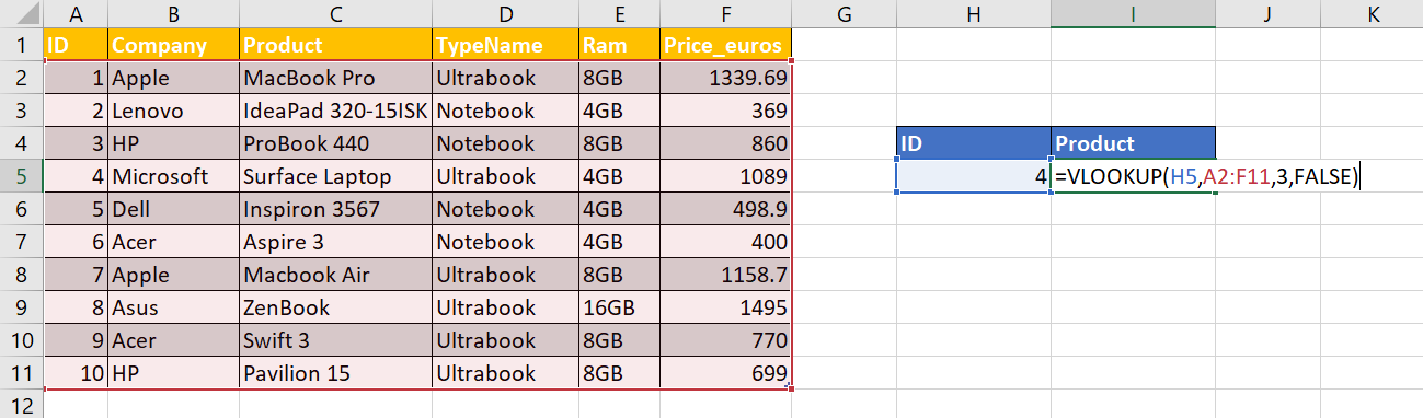
• We specify the location of the table in the second argument. As you can see, the table location is A2:F11.
• The third argument specifies the Column Index number. This tells us what value should be returned from the row that we are looking up for. In the example, the product column is 3.
• The last argument is a Boolean Expression. Here, the value is set to FALSE for the VLOOKUP function to return an exact match for the value. An N/A error is displayed in case the exact value is not found. 

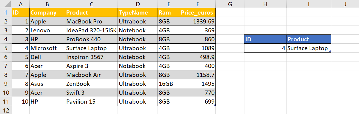
With the help of VLOOKUP in Excel, we can look for an approximate match as well. You will learn this in the next section.

How To Find Approximate Match Using VLOOKUP?

Approximate Match works by finding the next largest value that is lesser than the lookup value, which we specify. 

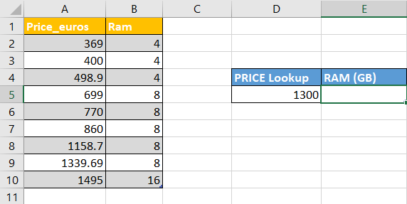
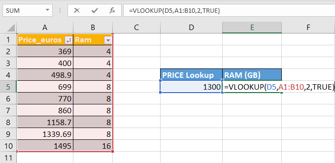
In the example below, we use the VLOOKUP function to find out how much RAM specification a laptop priced 1300 EUR has. Also, we know this value is not present in the table. So, let’s use the Approximate Match to find the solution. We need to sort the first column in ascending order. If not, VLOOKUP will return incorrect values.

• First, copy the price and RAM details to a new location, and specify your lookup value. Here, the lookup value is $1300. 

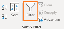
Next, select your data range and click on the filter option to sort the values of the first column based on ascending order. After you click on the filter option, you will see the filter buttons enabled on your column headers. 

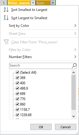
• Filter the price details in ascending order. Click on OK.

• Now, enter your VLOOKUP formula. The first argument will be the VLOOKUP value. The second argument specifies the table range. In the third argument, we give the column number, so that values for that column are returned. Finally, the last argument is set to TRUE. This will allow the VLOOKUP function to find an approximate match for the value.

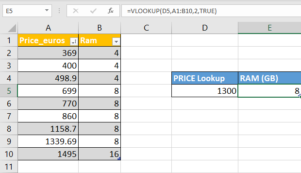
• After entering the formula, press enter. The value returned, in this case, is 8GB for the price of $1300.

Let’s proceed to the next section and understand how to use VLOOKUP for multiple criteria. 

B

How to Use VLOOKUP for Multiple Criteria?

With a helper column, you can give multiple criteria that the VLOOKUP genetically cannot handle. In our example, we will be calculating the price based on both company and product.

For example, if we have to look up the price of an Apple MacBook Pro, where the company name and product name are in two different columns, we use a helper column. This column will store the concatenated values of both columns.

Follow the steps below to perform VLOOKUP with multiple criteria.

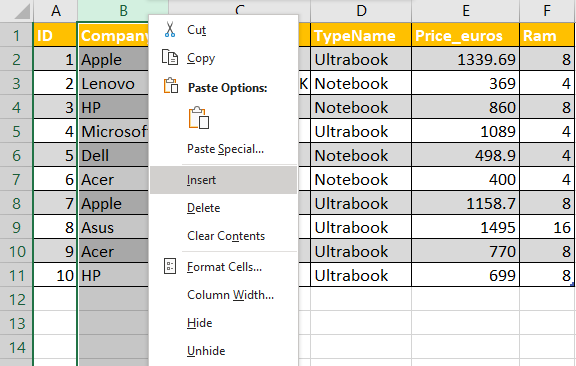
• First, right-click on a column header and click on Insert. This will help you insert a column to the left of the Company column. Name it as ‘Company & Product’. 

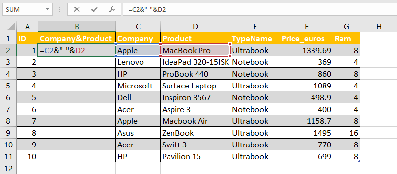
• On creating the helper column, enter the formula =C2&”-”&D2. Then, drag the formula down to the rest of the cells in the column.  

• On creating the concatenated column successfully, we can now look for the value. Here, we look for the price of an Apple MacBook Pro.
• So, we enter the formula =VLOOKUP(B15&”-”&C15,B1:G11,5,FALSE)

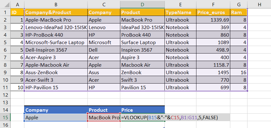
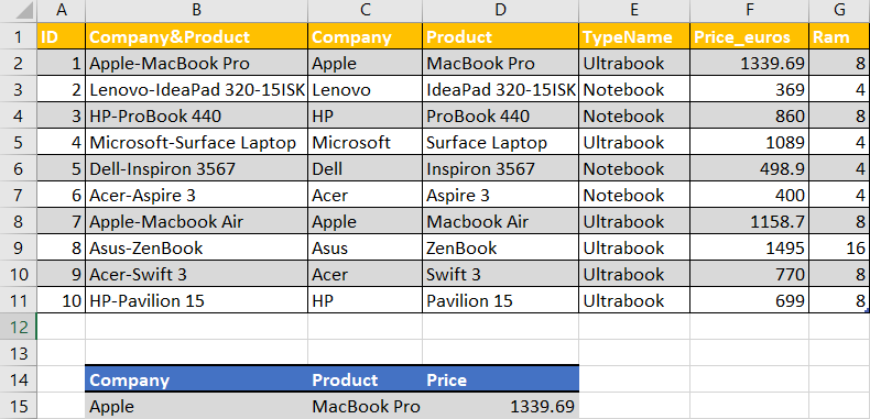
• The first parameter helps to concatenate the lookup value, i.e., B15&”-” &C15. We can also use the concatenate formula, i.e., CONCATENATE(B15,”-“,C15). The second parameter is the table range. The third parameter specifies the column index, which returns a value from that column. The final parameter is FALSE, as we are looking for an Exact Match. On pressing enter, the price will be returned as follows.

How to Use VLOOKUP Across Multiple Sheets 

Using VLOOKUP across multiple sheets in Excel can help you find and retrieve data from a large dataset spread across multiple worksheets. Here are the steps:

1. Open the worksheet that contains the data you want to retrieve and the worksheet where you want to place the lookup results.
2. Identify the common field in both worksheets that you can use as a reference point for your lookup, which could be a unique identifier, such as a product code or a customer ID.
3. In the worksheet where you want to place the lookup results, enter the VLOOKUP formula in the cell where you want to retrieve the data.
4. In the VLOOKUP formula, specify the lookup value, the range of cells where the lookup value is located in the source worksheet, the column index of the data you want to retrieve, and the range of cells that contain the source data across multiple sheets, separated by a comma.
5. Press Enter to see the lookup result in the cell.

Repeat the process for each lookup value and ensure that the common reference field in both worksheets is correctly aligned. With this method, you can easily retrieve data from multiple sheets in Excel using VLOOKUP.

Tips to Use VLOOKUP Function Efficiently 

When we enter an incorrect formula or add a wrong value somewhere the VLOOKUP function shows an error. Here are some tips that you must keep in mind while using VLOOKUP function – 

1. If you omit range_lookup from the VLOOKUP function, it will evaluate the non-exact matches as well. However, it will use an exact match if it exists in your data.
2. If the lookup column has duplicate values then it will only pick the first value. 
3. VLOOKUP is not case-sensitive. 
4. Adding a column after applying VLOOKUP formula will show an error as hard-coded index values don’t change automatically on adding or deleting columns. 

Common Errors in VLOOKUP Function 

• #N/A! error – Occurs if the VLOOKUP function fails to find a match to the supplied lookup_value. 
• #REF! error – Occurs if when the col_index_num argument > number of columns in the supplied table_array; or the formula attempts to reference cells that do not exist. 
• #VALUE! error – Occurs if either:  The col_index_num argument is less than 1 or is not recognized as a numeric value; or The range_lookup argument is not recognized as one of the logical values TRUE or FALSE.

This is all you need to know about VLOOKUP in Excel.

Limitations of VLOOKUP in Excel

Here are some limitations of VLOOKUP in Excel:

• VLOOKUP only looks for a match in the first column of the lookup range. This means you cannot use it to search for a value in a different column of the lookup range.
• VLOOKUP is not case-sensitive, so it may return incorrect results if the lookup value is in a different case than the data in the lookup range.
• VLOOKUP only returns the first matching value in the lookup range. This means that if there are multiple occurrences of the lookup value in the lookup range, VLOOKUP will only return the first one.
• VLOOKUP can only handle data that is sorted in ascending order. This means that if the data is not sorted, VLOOKUP may return an incorrect result.
• VLOOKUP cannot handle data that contains errors or blank cells. If the lookup range contains errors or blank cells, VLOOKUP may return an incorrect result.
• VLOOKUP is not very flexible when changing the lookup value or range. If you need to change the lookup value or the lookup range, you must manually update the VLOOKUP formula

Source:- https://www.simplilearn.com/tutorials/excel-tutorial/vlookup-in-excel